ggplot2: Plot Inside A Plot
May 8, 2009
Charts & Graphs blog demonstrates how to embed one chart within another chart using base graphics.
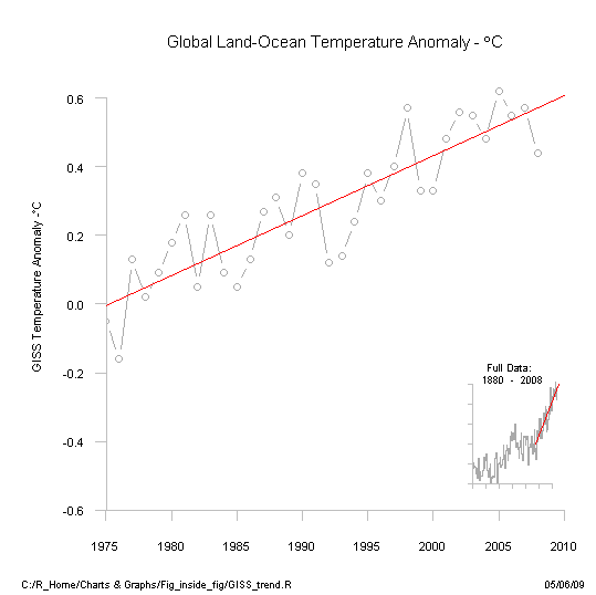
A similar chart can be drawn using ggplot2.
Data Import
The datafile used will be downloaded from the web, and as it includes some unnecessary information this needs to be stripped out first.
> library(ggplot2)
> file <- c("http://data.giss.nasa.gov/gistemp/graphs/Fig.A2.txt")
> rows <- length(readLines(file)) - 5
> df <- read.table(file, skip = 4, nrows = rows,
     header = FALSE, na.strings = "*")
> df <- df[, 1:2]
> names(df) <- c("year", "mean")
|
Theming
The standard black-white theme is edited to remove the panel background and the gridlines.
> theme_white <- function() {
     theme_update(panel.background = theme_blank(),
         panel.grid.major = theme_blank())
 }
> theme_set(theme_bw())
> theme_white()
|
Plot preparation
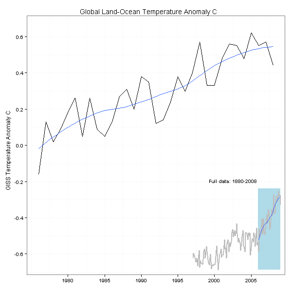
The main plot only shows a subset of the full data, whilst the small subplot shows the full trend and highlights the period shown in the main plot.
> p <- ggplot(df, aes(year, mean)) + labs(x = NULL,
     y = ("GISS Temperature Anomaly C")) + ylim(-0.65,
     0.65)
> mainplot <- p %+% subset(df, year > 1975) +
     geom_line() + geom_smooth(se = FALSE) +
     opts(title = "Global Land-Ocean Temperature Anomaly C")
|
> p1 <- p + geom_rect(aes(xmin = 1975, xmax = max(year),
     ymin = min(mean, na.rm = TRUE), ymax = 0.65),
     fill = alpha("lightblue", 0.2)) + scale_x_continuous(breaks = NA) +
     scale_y_continuous(breaks = NA) + labs(y = NULL) +
     opts(title = "Full data: 1880-2008") +
     opts(plot.title = theme_text(face = "bold")) +
     opts(panel.border = theme_blank())
|
> subplot <- p1 + geom_line(colour = I("grey"),
     size = 0.8) + geom_smooth(se = FALSE, subset = .(year >
     1975))
|
> vp <- viewport(width = 0.4, height = 0.4, x = 1,
     y = unit(0.7, "lines"), just = c("right",
         "bottom"))
|
Printing the Full Plot
This function is defined primarily to make saving the final graph to file easier. Also note the use of theme_set() to specify a smaller font size for the subplot.
> full <- function() {
     print(mainplot)
     theme_set(theme_bw(base_size = 8))
     theme_white()
     print(subplot, vp = vp)
     theme_set(theme_bw())
 }
> full()
|
13 Comments
leave one →


LearnR
Another interesting comparison of base & ggplot2 graphic scripts.
I like how you handled the source data file. I hadn’t thought of the readline() technique.
I’ve been trying to figure out how to read this file:
http://data.giss.nasa.gov/gistemp/tabledata/GLB.Ts.txt
The repeating titles every 20 years has me stumped. Do you have a trick for reading this type of source data file into R?
Kelly O’Day
http://processtrends.com
http://chartsgraphs.wordpress.com
This is a very useful example I’d like to experiment with for some data I’m plotting. I have two problems, one which seems simple and the other less so.
I think that the command
df <- read.table("Fig.A2.txt", skip = 4, nrows = rows,
header = FALSE)
should be
df <- read.table(file, skip = 4, nrows = rows,
header = FALSE)
When I execute full(), I get the following error:
Error in Summary.factor(c(23L, 17L, 21L, 22L, 26L, 26L, 24L, 30L, 22L, :
min not meaningful for factors
In addition: There were 31 warnings (use warnings() to see them)
I think I've copied the statements fairly faithfully. Is it due to a difference in ggplot2 (now 2.11.0) from the version you originally used?
regards – David
Sorry for the late reply, have been away on holiday.
You are right, there was a mistake in the read.table command – this is fixed now.
Adding
na.strings = "*"to read.table should get you around the error – have edited the post as well.Thanks, that works perfectly.
regards – David
Hi:
Is strange I can’t have geom_rect display the ligthblue background. It seems that the ‘fill’ argument is being ignored. I tried other colous and it still shows a white background. I am using the latest ggplot2 version and R 2.11
As the dataset contains NAs, then adjusting the aes-call to ignore NAs (
min(mean, na.rm = TRUE)) fixes this problem – updated the post to reflect this.Thanks, It didn’t cross my mind checking for NA’s. By the way sorry for the typo above, colous should be colors. 😉
I’m being told by R- Error: could not find function “viewport”. I have ggplot2 library loaded. Any ideas?
You would neet to load grid as well.
library(grid)