ggplot2 Version of Figures in "Lattice: Multivariate Data Visualization with R" (Part 6)

This is the 6th post in a series attempting to recreate the figures in Lattice: Multivariate Data Visualization with R (R code) with ggplot2.

Previous parts in this series: Part 1, Part 2, Part 3, Part 4, Part 5.

---

Chapter 6 – Trivariate Displays

Topics covered:

• Three dimensional scatter plots
• Surfaces and two-way tables
• Level plots and contour plots
• Wireframe rendering
• Parameterized surfaces

Figure 6.1

> library(lattice) > library(ggplot2)

> quakes$Magnitude <- equal.count(quakes$mag, 4)

lattice

> pl <- cloud(depth ~ lat * long | Magnitude, data = quakes, + zlim = rev(range(quakes$depth)), screen = list(z = 105, + x = -70), panel.aspect = 0.75, xlab = "Longitude", + ylab = "Latitude", zlab = "Depth") > print(pl)

ggplot2

ggplot2 currently does not support true 3d surfaces.

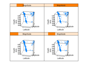
Figure 6.2

lattice

> pl <- cloud(depth ~ lat * long | Magnitude, data = quakes, + zlim = rev(range(quakes$depth)), panel.aspect = 0.75, + screen = list(z = 80, x = -70), zoom = 0.7, scales = list(z = list(arrows = FALSE, + distance = 2)), xlab = "Longitude", ylab = "Latitude", + zlab = list("Depth\n(km)", rot = 90)) > print(pl)

ggplot2

ggplot2 currently does not support true 3d surfaces.

Figure 6.3

lattice

> p <- cloud(depth ~ long + lat, quakes, zlim = c(690, + 30), pch = ".", cex = 1.5, zoom = 1, xlab = NULL, + ylab = NULL, zlab = NULL, par.settings = list(axis.line = list(col = "transparent")), + scales = list(draw = FALSE)) > npanel <- 4 > rotz <- seq(-30, 30, length = npanel) > roty <- c(3, 0)

> pl <- update(p[rep(1, 2 * npanel)], layout = c(2, npanel), + panel = function(..., screen) { + crow <- current.row() + ccol <- current.column() + panel.cloud(..., screen = list(z = rotz[crow], + x = -60, y = roty[ccol])) + }) > print(pl)

ggplot2

ggplot2 currently does not support true 3d surfaces.

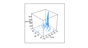
Figure 6.4

> state.info <- data.frame(name = state.name, long = state.center$x, + lat = state.center$y, area = state.x77[, "Area"], + population = 1000 * state.x77[, "Population"]) > state.info$density <- with(state.info, population/area)

lattice

> pl <- cloud(density ~ long + lat, state.info, subset = !(name %in% + c("Alaska", "Hawaii")), type = "h", lwd = 2, zlim = c(0, + max(state.info$density)), scales = list(arrows = FALSE)) > print(pl)

ggplot2

ggplot2 currently does not support true 3d surfaces.

Figure 6.5

> library("maps") > state.map <- map("state", plot = FALSE, fill = FALSE)

lattice

> panel.3dmap <- function(..., rot.mat, distance, xlim, + ylim, zlim, xlim.scaled, ylim.scaled, zlim.scaled) { + scaled.val <- function(x, original, scaled) { + scaled[1] + (x - original[1]) * diff(scaled)/diff(original) + } + m <- ltransform3dto3d(rbind(scaled.val(state.map$x, + xlim, xlim.scaled), scaled.val(state.map$y, ylim, + ylim.scaled), zlim.scaled[1]), rot.mat, distance) + panel.lines(m[1, ], m[2, ], col = "grey76") + }

> pl <- cloud(density ~ long + lat, state.info, subset = !(name %in% + c("Alaska", "Hawaii")), panel.3d.cloud = function(...) { + panel.3dmap(...) + panel.3dscatter(...) + }, type = "h", scales = list(draw = FALSE), zoom = 1.1, + xlim = state.map$range[1:2], ylim = state.map$range[3:4], + xlab = NULL, ylab = NULL, zlab = NULL, aspect = c(diff(state.map$range[3:4])/diff(state.map$range[1:2]), + 0.3), panel.aspect = 0.75, lwd = 2, screen = list(z = 30, + x = -60), par.settings = list(axis.line = list(col = "transparent"), + box.3d = list(col = "transparent", alpha = 0))) > print(pl)

ggplot2

ggplot2 currently does not support true 3d surfaces.

Figure 6.6

lattice

> env <- environmental > env$ozone <- env$ozone^(1/3) > env$Radiation <- equal.count(env$radiation, 4) > pl <- cloud(ozone ~ wind + temperature | Radiation, env) > print(pl)

ggplot2

ggplot2 currently does not support true 3d surfaces.

Figure 6.7

lattice

> pl <- splom(env[1:4]) > print(pl)

ggplot2

> pg <- plotmatrix(env[1:4]) > print(pg)

Figure 6.8

> fm1.env <- lm(ozone ~ radiation * temperature * wind, + env) > fm2.env <- loess(ozone ~ wind * temperature * radiation, + env, span = 0.75, degree = 1) > fm3.env <- loess(ozone ~ wind * temperature * radiation, + env, parametric = c("radiation", "wind"), span = 0.75, + degree = 2) > library("locfit") locfit 1.5-4 2007-11-27 > fm4.env <- locfit(ozone ~ wind * temperature * radiation, + env) > w.mesh <- with(env, do.breaks(range(wind), 50)) > t.mesh <- with(env, do.breaks(range(temperature), 50)) > r.mesh <- with(env, do.breaks(range(radiation), 3)) > grid <- expand.grid(wind = w.mesh, temperature = t.mesh, + radiation = r.mesh) > grid[["fit.linear"]] <- predict(fm1.env, newdata = grid) > grid[["fit.loess.1"]] <- as.vector(predict(fm2.env, newdata = grid)) > grid[["fit.loess.2"]] <- as.vector(predict(fm3.env, newdata = grid)) > grid[["fit.locfit"]] <- predict(fm4.env, newdata = grid)

lattice

> pl <- wireframe(fit.linear + fit.loess.1 + fit.loess.2 + + fit.locfit ~ wind * temperature | radiation, grid, + outer = TRUE, shade = TRUE, zlab = "") > print(pl)

ggplot2

ggplot2 currently does not support true 3d surfaces.

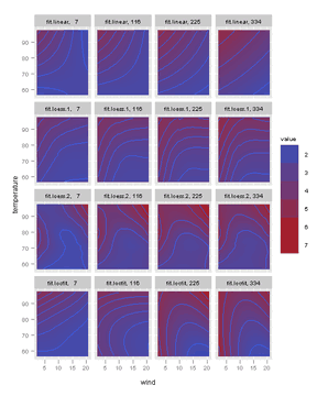
Figure 6.9

lattice

> pl <- levelplot(fit.linear + fit.loess.1 + fit.loess.2 + + fit.locfit ~ wind * temperature | radiation, data = grid) > print(pl)

ggplot2

> grid.m <- melt(grid, id.vars = 1:3)

> pg <- ggplot(grid.m, aes(wind, temperature, z = value, + fill = value)) + facet_wrap(~variable + radiation) + + geom_tile() + geom_contour() > print(pg)

Figure 6.10

lattice

> pl <- contourplot(fit.locfit ~ wind * temperature | radiation, + data = grid, aspect = 0.7, layout = c(1, 4), cuts = 15, + label.style = "align") > print(pl)

ggplot2

> pg <- ggplot(grid[, c(1:3, 7)], aes(wind, temperature, + z = fit.locfit)) + geom_contour() + facet_grid(radiation ~ + ., labeller = label_both) + opts(aspect.ratio = 1) > print(pg)

Note	Contour labeling not easily accomplished.

Figure 6.11

lattice

> plot(levelplot(volcano), split = c(1, 1, 1, 3), more = TRUE) > plot(contourplot(volcano, cuts = 20, label = FALSE), + split = c(1, 2, 1, 3), more = TRUE) > plot(wireframe(volcano, panel.aspect = 0.7, zoom = 1, + lwd = 0.01), split = c(1, 3, 1, 3), more = FALSE)

ggplot2

> library(ggextra)

Note	To install this package directly within R type: install.packages("ggextra", repos="http://R-Forge.R-project.org")

> p <- ggplot(melt(volcano), aes(x = X1, y = X2, z = value, + fill = value)) > p1 <- p + geom_tile() > p2 <- p + geom_contour(bins = 20) > print(arrange(p1, p2, ncol = 1)) [1] 3

Note	ggplot2 currently does not support true 3d surfaces.

Figure 6.12

> data(Cars93, package = "MASS") > cor.Cars93 <- cor(Cars93[, !sapply(Cars93, is.factor)], + use = "pair")

lattice

> pl <- levelplot(cor.Cars93, scales = list(x = list(rot = 90))) > print(pl)

ggplot2

> pg <- ggplot(melt(cor.Cars93), aes(X1, X2, fill = value)) + + geom_tile() + opts(axis.text.x = theme_text(lineheight = 0.9, + colour = "grey50", hjust = 1, angle = 90)) + opts(aspect.ratio = 1) > print(pg)

Figure 6.13

> ord <- order.dendrogram(as.dendrogram(hclust(dist(cor.Cars93))))

lattice

> pl <- levelplot(cor.Cars93[ord, ord], at = do.breaks(c(-1.01, + 1.01), 20), scales = list(x = list(rot = 90))) > print(pl)

ggplot2

> lvls <- rownames(cor.Cars93)[ord] > cor.Cars93.m <- melt(cor.Cars93) > cor.Cars93.m$X1 <- factor(cor.Cars93.m$X1, levels = lvls) > cor.Cars93.m$X2 <- factor(cor.Cars93.m$X2, levels = lvls)

> pg <- pg %+% cor.Cars93.m > print(pg)

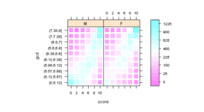
Figure 6.14

> data(Chem97, package = "mlmRev") > Chem97$gcd <- with(Chem97, cut(gcsescore, breaks = quantile(gcsescore, + ppoints(11, a = 1)))) > ChemTab <- xtabs(~score + gcd + gender, Chem97) > ChemTabDf <- as.data.frame.table(ChemTab)

lattice

> tick.at <- pretty(range(sqrt(ChemTabDf$Freq)))

> pl <- levelplot(sqrt(Freq) ~ score * gcd | gender, ChemTabDf, + shrink = c(0.7, 1), colorkey = list(labels = list(at = tick.at, + labels = tick.at^2)), aspect = "iso") > print(pl)

ggplot2

> pg <- ggplot(ChemTabDf, aes(score, gcd, fill = Freq)) + + facet_grid(~gender) + geom_tile() + scale_fill_gradient(trans = "sqrt") > print(pg)

Figure 6.15

> library("latticeExtra")

lattice

> pl <- cloud(Freq ~ score * gcd | gender, data = ChemTabDf, + screen = list(z = -40, x = -25), zoom = 1.1, col.facet = "grey", + xbase = 0.6, ybase = 0.6, par.settings = list(box.3d = list(col = "transparent")), + aspect = c(1.5, 0.75), panel.aspect = 0.75, panel.3d.cloud = panel.3dbars) > print(pl)

ggplot2

ggplot2 currently does not support true 3d surfaces.

Figure 6.16

> library("copula") > grid <- expand.grid(u = do.breaks(c(0.01, 0.99), 25), + v = do.breaks(c(0.01, 0.99), 25)) > grid$frank <- with(grid, dcopula(frankCopula(2), cbind(u, + v))) > grid$gumbel <- with(grid, dcopula(gumbelCopula(1.2), + cbind(u, v))) > grid$normal <- with(grid, dcopula(normalCopula(0.4), + cbind(u, v))) > grid$t <- with(grid, dcopula(tCopula(0.4), cbind(u, v)))

lattice

> pl <- wireframe(frank + gumbel + normal + t ~ u * v, + grid, outer = TRUE, zlab = "", screen = list(z = -30, + x = -50), lwd = 0.01) > print(pl)

ggplot2

ggplot2 currently does not support true 3d surfaces.

Figure 6.17

lattice

> pl <- wireframe(frank + gumbel + normal + t ~ u * v, + grid, outer = TRUE, zlab = "", screen = list(z = -30, + x = -50), scales = list(z = list(log = TRUE)), + lwd = 0.01) > print(pl)

ggplot2

ggplot2 currently does not support true 3d surfaces.

Figure 6.18

> kx <- function(u, v) cos(u) * (r + cos(u/2) * sin(t * + v) - sin(u/2) * sin(2 * t * v)) > ky <- function(u, v) sin(u) * (r + cos(u/2) * sin(t * + v) - sin(u/2) * sin(2 * t * v)) > kz <- function(u, v) sin(u/2) * sin(t * v) + cos(u/2) * + sin(t * v) > n <- 50 > u <- seq(0.3, 1.25, length = n) * 2 * pi > v <- seq(0, 1, length = n) * 2 * pi > um <- matrix(u, length(u), length(u)) > vm <- matrix(v, length(v), length(v), byrow = TRUE) > r <- 2 > t <- 1

lattice

> pl <- wireframe(kz(um, vm) ~ kx(um, vm) + ky(um, vm), + shade = TRUE, screen = list(z = 170, x = -60), alpha = 0.75, + panel.aspect = 0.6, aspect = c(1, 0.4)) > print(pl)

ggplot2

ggplot2 currently does not support true 3d surfaces.

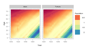
Figure 6.19

> data(USAge.df, package = "latticeExtra") > library("RColorBrewer")

lattice

> brewer.div <- colorRampPalette(brewer.pal(11, "Spectral"), + interpolate = "spline")

> pl <- levelplot(Population ~ Year * Age | Sex, data = USAge.df, + cuts = 199, col.regions = brewer.div(200), aspect = "iso") > print(pl)

ggplot2

> pg <- ggplot(USAge.df, aes(Year, Age, fill = Population)) + + facet_grid(~Sex) + geom_tile() + scale_fill_gradientn("Population", + colours = brewer.div(200)) + opts(aspect.ratio = 1) > print(pg)

About these ads